In a previous post, I discussed the physical
interpretation of digital music (and all digital audio) as both a time-varying
signal and a frequency-varying signal. This, of course, makes intuitive sense -
as we spend three or four minutes listening to a song, we can hear the guitars
and horns coming in and fading out, a singer intone the chorus of a song, etc.
At the same time, we appreciate the frequencies changing as well — the
singer hitting different notes, the instruments forming different chords.
Understanding the time and frequency behavior of auditory information is fairly
intuitive - in fact, one could even argue that visualizing the frequency-based
content is more informative than visualizing the time-based content.
Unfortunately, visual information does not operate in exactly the same way as
auditory information, and therefore understanding the time-frequency duality is
slightly more involved. However, with a few examples, we can generalize our
conceptual understanding of signals from time-varying signals to space-varying
signals.
Preface: How Do Digital Images Work?
You can feel free to skip this section if you’re already familiar with how
digital images are stored and represented on a computer. If not, don’t worry
— it’s pretty straightforward.
Digital images, which is to say bitmap images, are fundamentally composed of
pixels. (Bitmap images should not be
confused with vector images, which are not composed of pixels.) Pixels are
simply little boxes containing some combination of colors placed into a grid;
when viewing a grid of several hundred, several thousand, or (especially today)
several million at once, the pixels taken together appear as an image. (For
you artists, this is exactly analogous to
pointillism, except with squares
instead of dots.)
Black and white images, which are simpler to think about and store, are
basically a grid of values, with the value in each element in the grid
representing a color. The purest black is the value 0, the purest white is the
value 255, and every whole number in between is a shade of gray. (Color images
are a bit more complex - they use the same 0 to 255 scale grid, but they use 3
grids each measuring Red, Green and Blue values. Each pixel is then the
depiction of the combination of Red, Green, and Blue at the corresponding
location in each grid. We can discuss the basic concepts of imaging without
worrying about color.) When a computer displays any image, it checks each pixel
value and displays the corresponding color. However, the images are still
fundamentally a grid of pixels.
The fact that digital images are composed of these myriad discrete, uniformly
distributed elements (pixels) is very important because these elements of color
and shade can be understood as approximations of a whole image. In fact, this is
what is meant by a digital image — the image contains digital data
(digital meaning containing a series of discrete and finite-values); these
digital data comprise the digital image.
Time-Varying Signals vs Space-Varying Signals
The concept of a time-varying signal really isn’t too hard to understand. At
every time, there is a value, and the value varies over time. Hence the name.
And that’s it.
Space-varying signals may sound bad, but they’re actually not much different
than time-varying signals. The main difference is in the physical meaning of the
signal — everything else is exactly the same.
For a space-varying signal, at every element in the “signal” there is a
value. Sound familiar? That’s how we defined digital images! At every row, for
each column, there is a value. Therefore, images are space-varying signals.
Actually, it’s a little more complex than that. Because there’s both a row and a
column needed to identify a value in an image, images are actually varying in
two dimensions at once. This is a bit more advanced than our time-varying songs,
which only vary in time. Nevertheless, both conceptually and physically, they
each operate exactly the same way. This is immensely useful because the
techniques which worked on music will also work on images, although with a
different meaning.
What is the Frequency of Space?
If you recall how I explained a
lowpass filter
in the previous post, I stated that the idea is to keep the low frequencies of a
signal largely intact while trying to reject the higher frequencies of a signal.
In that context, “pumping up the bass” is accomplished with a low-pass filter.
At the time, I mentioned that much of the finer details of music is contained in
the upper frequencies of a song, without going into too much depth. This is an
appropriate time to expand upon that concept.
The physical/mathematical meaning of frequency is the rate at which some
repetitive event repeats itself. (For example, a birthday has a frequency of
once a year, but the 31st day of the month has a frequency of 9 times a year.)
An important result of mathematics states that not only is it possible, but it
is also meaningful to generalize that statement to say that even events which
never repeat have frequency. The correct interpretation of frequency then
becomes how quickly something occurs, rather than how often it repeats. This
generalized definition does not contradict the previous definition —
repeating events also have a frequency; the slower the rate of occurrence of an
event, the lower its frequency. Emphasis on “rate”.
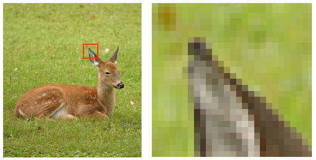
Believe it or not, this approach to understanding frequencies actually allows us
to interpret images as having frequencies. Recall that an image is fundamentally
just a grid of values, and frequency is how quickly something happens. What if I
said frequency is the rate at which adjacent pixels spike in value? A slow
change in values across several pixels would have a low frequency because it
happens slowly, and a rapid spike in value across only a few pixels would then
have a high frequency because it happens quickly. Of course, we would have to
measure these frequencies in two dimensions, because the original image was also
defined in dimensions. Nevertheless, we have discovered a powerful technique.
Frequency Filtering Images
With our broader understanding of frequency, we can begin to apply frequency-
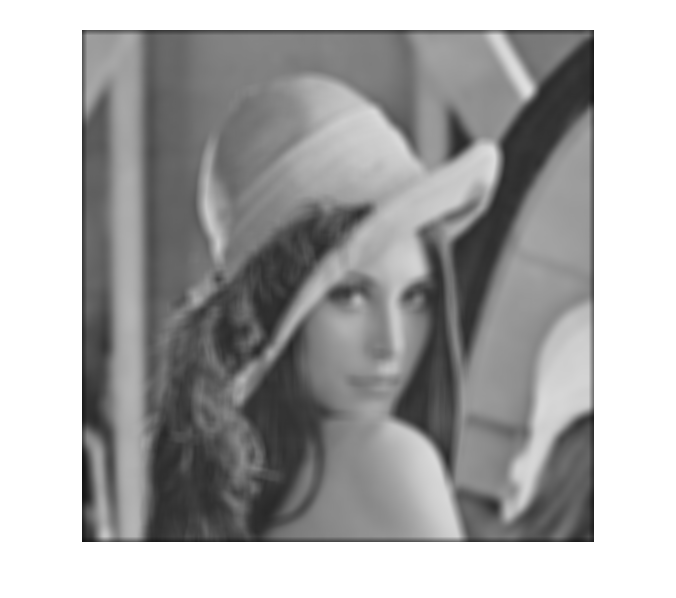
domain techniques to images. Perhaps it is best to start with an example. Below
is a black-and-white of the famous PG-version image of
Lena from November 1972,
and below that is a low-pass filtered version of it.

At first glance, the lower image appears badly blurred – and it is. Much
of the detail has been lost. However, take note of how smooth Lena’s skin in the
filtered image is, and how soft the edges in the picture are. These effects are
created by the filter. Low pass filtering remove the high frequency components
of an image. As explained above, the high frequency components are rapid and
extreme changes in value between nearby portions of pixels. Therefore, the low
pass filter removed things like the borders between objects and skin
imperfections, which have large local differences in pixel value. Think of it as
smoothing out the image.
Although the filtered image shown is an extreme example, this technique is
actually a standard in a Photoshop user’s repertoire. For instance, judicious
application of low-pass filtering to select portions of a picture of model’s
skin, for instance, goes a long way in creating the illusion of having flawless
skin.
Conclusion
There are many more applications of image processing than shown here, a great
deal of which require more advanced mathematics than I care to show here.
However, I hope I have given a taste of how a strong understanding of the
physics of digital images and audio allows us to enhance things to be more to
our liking.